Prefill is compute-bound, decode is bandwidth-bound, and KV cache is what really caps concurrency. The metrics, memory maths and tradeoffs behind serving.
Training runs get the headlines. Inference gets the electricity bill. A model is trained once and then answers requests for the rest of its life, which is why almost all real accelerator time — hyperscaler and homelab alike — goes to inference, not gradient descent. If you run a model on your own hardware you have already taken the job, whatever your title says.
Inference engineering is the craft of turning a directory of weights into a service that meets a latency target at an acceptable cost. Much of that is ordinary backend work; what makes it a discipline of its own is that the workload has properties no web service has. A single request occupies an accelerator for seconds, not milliseconds. Its cost depends on both the length of its input and the length of its output, and those two costs have different shapes. Memory consumption grows while the request is in flight. And measured throughput on an identical deployment can differ by an order of magnitude depending on a batching setting most people never touch.
The skills are narrow enough to enumerate: computing a model's memory cost from its card; choosing a numeric format; configuring a serving engine; reasoning about batching, concurrency and queueing; sizing hardware from a workload description; benchmarking in a way that predicts production; and recognising the failure modes behind most incidents. This piece maps the territory.
Everything follows from two phases
A generation request runs in two phases with opposite performance characteristics. Almost every optimization exists because of this split, so get it exactly right.
Prefill processes the prompt. It is all available at once, so every token goes through the network in parallel as one large matrix multiplication per layer, doing a great deal of arithmetic on data already loaded. Operations per byte moved is high. Prefill is compute-bound: limited by how many FLOPs your hardware retires per second. Doubling the prompt roughly doubles prefill time, and it gets worse than linear once attention over a long context dominates.
Decode generates the output one token at a time. Token N+1 cannot be computed until token N exists, so there is no parallelism within a sequence. Here is the crucial part: to produce that one token, the accelerator must read every active weight in the model out of memory and into compute units. All of them. For one token. The arithmetic on each weight is trivial — a few multiply-accumulates against one vector — so compute sits idle waiting on memory. Decode is memory-bandwidth-bound.
That gives a back-of-envelope ceiling that holds up well in practice:
max single-stream tokens/sec = memory bandwidth (bytes/sec) / active weight bytes per token
A model with 18B active parameters in FP8 reads roughly 18 GB per token. On a machine with 1092 GB/s of aggregate bandwidth, that is about 60 tokens per second, ceiling, before overhead. No amount of compute helps; only bandwidth does.
Two consequences follow. Prefill and decode want different hardware, which is why some deployments separate them onto different node pools. And since decode leaves compute idle, other sequences' tokens ride along in the same weight read almost free — the economic basis of batching, and why aggregate throughput and single-stream latency move in opposite directions.
The metrics, defined precisely
Vague throughput claims are the main source of confusion. Pin these down.
Time to first token (TTFT) — request arrival to first token at the client: queue wait plus prefill, dominated by prompt length, and it governs whether an interface feels responsive.
Time per output token (TPOT), or inter-token latency — the steady-state gap between tokens during decode, the reciprocal of single-stream decode rate. 64 tokens per second is about 15.6 ms per token.
End-to-end latency — the whole request: e2e = TTFT + (N - 1) * TPOT for N output tokens. Long outputs are decode-dominated; a 60k-token context with a 200-token answer is prefill-dominated. Know which regime your traffic sits in before optimizing anything.
Throughput — tokens per second, and this is where people talk past each other. Single-stream throughput is what one user experiences; aggregate throughput is the total the server emits across all concurrent sessions. Different numbers, and they trade against each other.
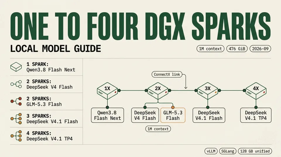
Community testing of a 2x DGX Spark deployment of Qwen3.8-Flash-Next makes the point: roughly 64 tokens per second single-stream, roughly 115 aggregate across 2–4 concurrent sessions. Concurrency raised total output by around 80 percent while cutting each user's rate — at four sessions, to near 29 each. Both numbers are correct. A vendor quoting only the aggregate describes a server; a user complaining about a slow chatbot describes the single stream.
So whenever you meet a throughput claim — including the roughly 800 tokens per second community testing reports for GLM-5.3-Flash in a tuned serving setup — the first question is: at what concurrency? A number with no batch size attached is not plannable.
Track goodput too: the throughput of requests that actually met your latency target.
Memory is the real budget
Accelerator memory, not compute, is what you run out of. Four things compete for it.
Weights. Parameter count times bytes per parameter. GLM-5.3-Flash at 320B parameters in FP8 lands at approximately 328 GB. Qwen3.8-Flash in NVFP4 comes to approximately 135 GB, which is why that deployment needs two 128 GB DGX Spark units rather than one.
KV cache. Every processed token leaves key and value tensors for every layer, so attention over the growing sequence need not recompute the past:
kv_bytes_per_token = 2 * num_layers * num_kv_heads * head_dim * bytes_per_element
kv_total = kv_bytes_per_token * sum(context length of each active sequence)
The leading 2 is keys and values. num_kv_heads is usually far smaller than the attention head count, because grouped-query attention exists to shrink this term. Read the config file; do not guess.
KV cache grows linearly in context length and linearly in the number of concurrent sequences. It is not a fixed overhead allocated once but a per-request, per-token tax accumulating as the conversation continues — and it, not your weights and not your FLOPs, is what actually caps concurrency. A deployment that comfortably serves forty users at 4k context may serve five at 64k.
Activations. Transient per-layer working memory. Modest during decode; substantial during prefill and proportional to tokens prefilled at once — the knob chunked prefill exposes.
Framework overhead. Accelerator context, communication buffers, captured graphs, fragmentation. Reserve for it rather than meeting it at 3 a.m.
The planning identity: kv_budget = total_memory - weights - activations - overhead. Your concurrency ceiling is that budget divided by per-sequence KV cost.
Batching, and why continuous batching won
Because decode is bandwidth-bound, one weight read serves many sequences. Batch size 8 costs barely more wall-clock time per step than batch size 1, so aggregate throughput scales near-linearly until memory bandwidth or KV capacity saturates.
Static batching collects a batch, runs it, returns it. Simple and wasteful, because sequences finish at different times: one request generating 900 tokens holds the whole batch open while seven that finished at 40 sit idle. Utilization collapses to the longest member.
Continuous batching (in-flight batching) works at the granularity of one decode step: when a sequence emits its end-of-sequence token it leaves the batch immediately and a queued request takes the slot on the next step. No request waits on an unrelated one.
This is the single largest throughput win in serving, and it costs nothing in output quality. vLLM, SGLang and TensorRT-LLM all implement it; verifying it is on is the first thing to do.
The honest tradeoff: larger batches mean higher aggregate tokens per second, slower per-user generation, and longer queue waits when a big prefill blocks the scheduler. Most engines expose maximum concurrent sequences and maximum batched tokens; those are your dials, and the right setting is whatever maximises goodput.
The core optimizations
Quantization. Does: stores weights — and sometimes activations and KV cache — in fewer bits: FP8, INT8, NVFP4, or a 4-bit weight-only scheme. Helps: always, on bandwidth-bound decode — fewer bytes per weight means proportionally faster generation and more room for KV cache. Costs: accuracy, unevenly. Degradation surfaces first in long-context reasoning, structured output and rarer languages while short chat answers look untouched. Format choice is its own decision: calibration data, hardware support, whether KV cache is quantized too.
PagedAttention and KV paging. Does: stores KV cache in fixed-size blocks behind an indirection table instead of one contiguous per-sequence reservation — virtual memory paging, applied to attention. Helps: always, especially with variable-length requests: contiguous allocators reserve for the worst case and waste most of it, while paging cuts fragmentation and raises concurrency for the same memory. Costs: a little indirection overhead, already absorbed by the engines that ship it.
Prefix caching. Does: spots that many requests share a leading prefix — a system prompt, a few-shot block, a document asked repeated questions about — and reuses the computed KV blocks instead of re-prefilling. Helps: enormously wherever prompts share structure; a 2,000-token system prompt removes 2,000 tokens of prefill from every request. Agent loops, resending a growing transcript each turn, benefit most. Costs: memory held by cached blocks, plus a cache policy. Two gotchas: matching is prefix-exact, so anything variable (a timestamp, a user id) at the top of the prompt defeats it entirely — put variable content last; and cached blocks compete with live sequences for the pool.
Speculative decoding and multi-token prediction. Does: attacks decode's serial dependency. A cheap drafter — a small model, an n-gram lookup, or an MTP head trained onto the main model — proposes k tokens, and the full model verifies all k in a single forward pass, because verifying a known candidate is parallel, just like prefill. Accepted tokens are kept; the first rejection discards the rest and generation resumes there. Done correctly, output is mathematically identical to standard decoding — a latency optimization, not an approximation. Helps: at low concurrency, where compute sits idle and verification is nearly free, and most on predictable text: code, structured formats, repetitive prose. Costs: drafter memory and complexity, and it can reduce throughput at high batch sizes, where compute is saturated and rejected drafts are wasted work. The 2x DGX Spark figures above used SGLang with MTP.
Chunked prefill. Does: splits a long prefill into slices and interleaves them with decode steps for other sequences. Helps: whenever long prompts and interactive sessions share a server. Without it, one 100k-token prefill monopolises the accelerator and every other stream stalls — visible as a spiky, bimodal TPOT distribution. Costs: slightly longer prefill for that request, and a chunk size to tune. It turns a latency disaster for many users into a small tax on one.
CUDA graphs and kernel fusion. Does: fusion merges adjacent operations into one kernel so intermediates stay in registers instead of round-tripping through memory; graph capture records a decode step as a replayable graph, removing per-kernel launch overhead. Helps: decode steps are short, so launch overhead is a real fraction of them — most visible on small models and fast hardware. Costs: capture time at startup, memory for graphs, and rigidity: graphs bind to specific shapes, so unusual batch sizes fall back to the slow path.
Parallelism, three kinds. Tensor parallelism (TP) splits individual weight matrices across devices, so each holds a shard of every layer. It divides memory and bandwidth pressure per device, which is why it speeds up decode, but it needs an all-reduce at every layer: fast interconnect required, and it degrades badly across slow links. Pipeline parallelism (PP) assigns whole layer ranges to devices; traffic is only boundary activations, so it tolerates slower links, but naive pipelines leave idle bubbles and per-device bandwidth pressure is unchanged. Expert parallelism (EP) distributes an MoE model's experts; traffic is the routed tokens themselves — load-dependent, bursty, easily unbalanced. In practice, combine: TP inside a fast-interconnect node, PP or EP across nodes.
Serving stacks, without a winner
vLLM — the general-purpose default: originated PagedAttention, broad model coverage, an OpenAI-compatible server, large community.
SGLang — strongest on structured generation, aggressive prefix caching (RadixAttention) and multi-token prediction. For agentic and structured workloads, or when you need MTP.
TensorRT-LLM — compiles an engine ahead of time for specific NVIDIA hardware and shapes: highest ceiling, least flexible, recompile on every model change.
llama.cpp — C++ with GGUF quantization, CPU and mixed CPU/GPU execution, wide hardware support including Apple Silicon. For one user, constrained hardware, or inference embedded in an app.
Ollama — packaging and model management over llama.cpp with a pull-and-run UX. For local development; it is not a multi-tenant production tier.
Selection criteria, in the order that usually decides it: does it support your architecture and quantization format; does it run on your hardware; does it do continuous batching and paged KV; does it cover the features you need (long context, vision, structured output, tool calling); and only then, benchmark numbers.
MoE: 18B active, 320B resident
Mixture-of-experts models are where most capacity planning goes wrong. GLM-5.3-Flash is 320B total parameters with 18B active. The router picks a small subset of experts per token, so compute per token resembles an 18B dense model — genuinely cheap.
But it can pick any expert, per token and per layer, so every expert must be resident in memory at all times. You pay 18B-scale compute and 320B-scale memory. That is the 328 GB FP8 footprint, and it does not shrink because only 18B are active.
Bandwidth sits in between, and that is the subtle part. Per token you stream only the active experts, so decode behaves like an 18B model. But at batch size 32 different sequences route to different experts, and the union touched per step climbs toward all of them. MoE efficiency is best at low batch sizes and erodes as concurrency rises — the opposite of dense-model intuition.
The rule: size memory by total parameters, size compute by active parameters, and measure bandwidth at your real concurrency.
A worked capacity plan
Target: 20 concurrent users, 32k context each, TTFT at or below 2 seconds, generation at or above 20 tokens per second per user. Candidate: Qwen3.8-Flash in NVFP4 on 2x DGX Spark, 256 GB total.
Step 1 — memory. Weights take approximately 135 GB. Reserve, say, 15 GB for activations, buffers and overhead. KV budget: 256 - 135 - 15 = 106 GB.
Step 2 — concurrency ceiling. Compute kv_bytes_per_token from the config with the formula above. Suppose it works out to 64 KB per token — an illustrative placeholder; substitute your model's real number. At 32k context a full sequence holds 32,768 * 64 KB = 2.1 GB, so 106 / 2.1 is about 50 sequences at full context. Twenty users fits with headroom, which matters: contexts grow and prefix cache blocks need room.
Step 3 — decode rate. Community testing of this class of deployment reports roughly 64 tokens per second single-stream and 115 aggregate at 2–4 concurrent; the data does not support extrapolating to 20. Treat it as a roofline problem instead: aggregate decode is capped by bandwidth divided by active bytes per token, and 20 users at 20 tokens per second needs 400 tokens per second aggregate. If the roofline for your hardware and format sits comfortably above that, go measure. If it sits near or below, you already have your answer.
Step 4 — TTFT. TTFT = queue_wait + prompt_tokens / prefill_rate. Measure prefill_rate on one unit with a representative prompt; being compute-bound, it is stable. Check that the queue does not dominate at your arrival rate, and enable chunked prefill so one long prompt cannot stall everyone else's decode.
Step 5 — scale, if needed. Two paths. Wider tensor parallelism: 4x DGX Spark at TP=4 gives roughly 1092 GB/s aggregate bandwidth, raising the single-stream ceiling but adding an all-reduce per layer. Or replicas: two independent 2-unit servers behind a load balancer double aggregate throughput at no interconnect cost and no latency change. If your problem is aggregate throughput, add replicas. Add tensor parallelism only when a single request must go faster, or when the model does not fit.
Note the shapes: that four-unit cluster reaches roughly 1092 GB/s across four boxes, while a 512 GB M5 Ultra is roughly 1200 GB/s in one box with no interconnect. For decode the single box is the better shape; the four-box cluster has four times the compute and wins prefill-heavy work. Match the machine to the dominant phase.
Benchmarking honestly
Most published inference numbers are useless to you, not because they are dishonest but because they came from conditions you will never reproduce.
Measure on your own prompt distribution. Input and output lengths drive everything. A benchmark with 128-token inputs and outputs says nothing about a RAG service with 40k inputs and 300-token outputs. Sweep concurrency 1, 2, 4, 8, 16, 32 and plot aggregate throughput against p95 latency; the knee is your operating point.
Report percentiles, not means. Mean TTFT hides exactly what users complain about. Publish p50, p95 and p99 for TTFT and TPOT. A bimodal TPOT distribution is a diagnosable signal: long prefills are blocking decode, and chunked prefill is the fix.
Separate prefill from decode. Report TTFT and TPOT separately, with the token counts that produced them. A single tokens-per-second number conflates two bottlenecks and is not actionable.
Warm up. The first requests pay for graph capture, memory pool growth, kernel autotuning and an empty prefix cache. Discard them.
State your concurrency. Every number needs a batch size beside it. Vendor figures are often measured at batch sizes that maximise aggregate throughput and destroy per-user latency — real numbers, irrelevant configuration.
Failure modes you will meet
OOM at long context that passed at short context. Weights are constant; KV cache is not — it scales with context and concurrency, so a load test with 2k prompts told you nothing about 64k prompts. Configure maximum context and concurrent sequences so the worst case fits, rather than letting production find the limit.
Throughput collapse from KV thrashing. When KV memory is exhausted, engines preempt: a running sequence is evicted, then recomputed or swapped back later. Under pressure that becomes a cycle of eviction and recomputation burning capacity on repeated work, and throughput falls off a cliff instead of degrading gracefully. Admission control — refusing or queueing what you cannot serve — beats thrashing. Treat preemption counts and KV utilization as first-class metrics.
A quantization that passes chat evals but breaks structured output. Quantization error concentrates in low-probability tail distinctions: responses stay fluent while JSON schema conformance, function-call formatting and long-chain arithmetic quietly degrade. Evaluate on the task you actually run, scoring schema validity and tool-call correctness, not chat quality.
Cold start on autoscaled deployments. Loading hundreds of gigabytes of weights, initialising the engine, capturing graphs and warming the prefix cache takes minutes, so scale-to-zero is a poor fit. Keep a warm floor, pre-stage weights on local NVMe, and scale on trends rather than instantaneous queue depth.
Where to go next
Four sub-topics carry the remaining depth. Quantization formats — how FP8, NVFP4, INT8 and the GGUF and AWQ families differ in calibration needs, hardware support and failure behaviour. KV cache mathematics — per-token footprint from a config file, grouped-query attention, KV quantization, and the arithmetic of long-context serving. Engine selection and tuning — mapping a workload to a stack, then finding the scheduler settings that maximise goodput. Multi-node topology — how TP, PP and EP compose across interconnects, and when a second replica beats a wider parallel group.
Work through those with the two-phase model in hand and the field stops looking like a bag of tricks. Prefill is compute, decode is bandwidth, KV cache is the budget, batching is the lever. Almost everything else is a consequence.