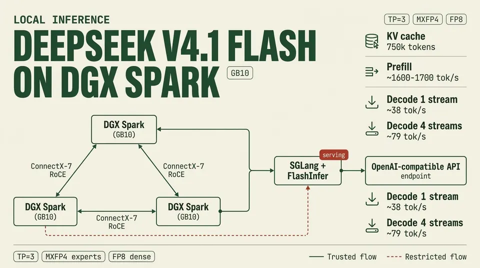
A 135 GB model against a 128 GB box forces a cluster. Here is the decision order, the parallelism maths, and what the interconnect really costs per token.
Qwen3.8-Flash in NVFP4 lands at approximately 135 GB of weights. A DGX Spark is a 128 GB unit. The gap is about 7 GB, roughly five percent, and no flag closes it. You cannot leave the last few layers on disk and keep a usable decode rate, and you cannot trim the tail of a weight tensor. The model either resides in memory or it does not.
That five percent is the cheapest possible trigger for the most expensive possible decision. The answer is not a bigger box, it is a second box, and a second box is a cluster: a collective library, an interconnect, a parallelism strategy, two driver stacks in lockstep, and a failure domain that runs through a cable. When is a second node genuinely required, how do you choose the strategy and its degree, what does the wire cost, and how do you size a 2x or 4x cluster?
Exhaust the single-box answers first
Multi-node is a real step up in complexity and belongs second, not first. Stop at the first line that clears your quality bar.
- A different model. Compare against the next model down in the family; a smaller sibling that passes your evaluation set keeps single-box failure behaviour.
- Quantization. The largest lever on weight footprint, and roughly linear. The saving is only real if a fast kernel exists for that format on your hardware, since an unoptimised kernel can decode slower than the same model on two nodes. Evaluate quality on your own task: quantization damage is uneven across capabilities.
- Context length. On long-context deployments the KV cache, not the weights, is the swing factor. Provisioning 900k when your documents are 40k buys nodes to hold cache you never fill.
- Concurrency. Every session is another KV allocation. One stream instead of eight is a large saving, often an honest description of an internal tool.
- Offload. Keeps the model on one box and destroys decode latency, since every token waits on the slowest tier holding a weight. Fine for overnight batch, useless interactively.
- A second node, once the model you need, at the precision that preserves quality, with the required context and concurrency, does not fit one box.
The 135 GB case fails step 2 if NVFP4 is already the fastest format you have kernels for, and fails steps 3 and 4 however you set them: the weights exceed 128 GB before a single token of cache exists. That is the signature of a genuine multi-node requirement: the weights, not the workload, overflow.
The four ways to split a model
Tensor parallelism
TP splits individual weight matrices across devices. A linear layer with output dimension H becomes N shards of H/N columns; each rank computes a partial result and the shards are recombined. In the standard transformer layout that means an all-reduce after the attention output projection and another after the MLP down projection: two collectives per layer, per forward pass, on every device. That makes TP the most interconnect-hungry strategy by a wide margin, and the best at preserving single-stream latency, since every device works the same token at once.
TP degree normally wants to divide the attention head count evenly, since heads are the natural shard boundary and a degree that does not divide them forces uneven shards, padding, or a fallback path. Head counts are almost always powers of two, so TP=2 and TP=4 are the common choices and odd degrees cause trouble. Grouped-query attention adds a constraint: a TP degree above the KV head count makes the runtime replicate KV across ranks, so you pay for the same cache twice.
Pipeline parallelism
PP splits by layer. Node 0 holds layers 0 through k, node 1 the rest, and activations hand off between stages. Communication volume is tiny next to TP, because only the boundary activation crosses the wire, once per microbatch. The cost is the bubble: with P stages and M microbatches in flight the idle fraction is approximately (P - 1) / (M + P - 1), so two stages and one request is 50 percent idle. PP rewards throughput and punishes single-user interactive work.
Expert parallelism
EP applies to mixture-of-experts models and gives each device a subset of experts outright. Routing traffic replaces weight traffic: tokens go to the device holding their chosen expert with an all-to-all, and results return with a second. That volume scales with tokens times hidden size rather than weight size, usually far smaller than a TP all-reduce over the same layer. The failure mode is imbalance: a hot expert makes its host the pace-setter while the others wait.
Data parallelism
Data parallelism runs full replicas and splits requests across them. It is persistently confused with the others, so state it plainly: data parallelism does not let you run a bigger model. Every replica needs the entire weight set in its own memory. Two Sparks running data-parallel give you two 128 GB boxes and twice the throughput on models that already fit one. They will not run the 135 GB model.
Combining them
Real deployments compose these: TP first inside the fastest communication domain, then EP if the model is MoE, then PP across the slowest links, and data parallelism on top as replicas. Put the chattiest strategy on the fattest pipe.
Memory arithmetic across nodes
Two 128 GB nodes are not a 256 GB machine. TP splits weights roughly evenly, but each node still budgets for its weight share, the non-sharded weights, an activation workspace, its KV cache share, framework and driver overhead, and the OS.
The weight share is W/N, but only approximately: embeddings and the output head are often replicated or sharded on a different axis, and runtimes keep replicated collective buffers.
Work the 135 GB model on two nodes. The weight share is 67.5 GB per node, so 135 GB of the 256 GB nameplate is spoken for and 121 GB is gross headroom. Subtract per-node overhead: OS, runtime, driver context, collective buffers, and the activation workspace, which scales with the largest batch times sequence chunk you prefill. Call that X GB per node and cluster headroom is 121 minus 2X: about 101 GB of usable pool at X = 10, about 81 GB at X = 20. Measure your own X: overhead is charged per node, so the curve is flatter than the nameplate suggests. What that headroom buys:
bytes per token = 2 x layers x kv_heads x head_dim x bytes_per_element
max context tokens = KV pool / bytes per token
max concurrent sessions = KV pool / (tokens per session x bytes per token)
The factor of two is K and V. Under TP, KV heads shard across ranks when the head count divides the degree, so the pool is additive. Context and concurrency draw on that one pool, which is the whole trade: doubling concurrency halves the context each session can have. A cluster sized for one 900k-token session is not one sized for ten 90k-token sessions: the second also needs ten times the peak workspace.
Bandwidth is the currency
Decode is memory-bandwidth-bound, not compute-bound. One token requires reading every weight the forward pass touches while doing little arithmetic per byte, so a batch-one decode step sits far below the arithmetic intensity at which FLOPS become the limit. Aggregate memory bandwidth therefore predicts token rate better than any FLOPS figure, so FLOPS comparisons mislead for serving even when they are right for training.
tokens per second is at most: aggregate bandwidth / bytes touched per token
Community testing reports put 4x DGX Spark at TP=4 at roughly 1092 GB/s aggregate memory bandwidth. A 512 GB M5 Ultra is roughly 1200 GB/s, and testers describe the two as almost identical on what matters. Take that both ways: if aggregate bandwidth is comparable, bandwidth is not the axis on which to choose. The differences sit elsewhere. Total memory capacity sets the largest model you can hold; interconnect topology decides how much of that aggregate you realise; software maturity determines which kernels and quantization formats are production-ready; and power and footprint is four units plus a switch against one chassis.
The caution the arithmetic hides: aggregate bandwidth across nodes is not equivalent to the same bandwidth in one address space. A single 512 GB machine reads any byte at full rate with no coordination. A four-node cluster reads its own shard at full rate and reaches everything else over the interconnect, and every TP collective serialises against that link. The aggregate figure is a sum of local bandwidths, available only while each node is reading its own memory.
The interconnect sets the ceiling for TP
For TP the link is the bottleneck, and it bites through latency as much as throughput. A ring all-reduce moves 2 x (N - 1) / N x S bytes through each device for a message of size S: 1.0 x S per device at N=2, and 1.5 x S at N=4. Per-device volume rises by half from two nodes to four, on top of more hops and a message that grows with batch size.
Two collectives per layer means 2L per forward pass for a model of L layers, and decode runs one forward pass per step:
per-token collective floor = 2 x L x round_trip_latency
Measure your own round trip and substitute it. At 60 layers, 120 collectives per token, a per-collective latency of T milliseconds costs 120 x T milliseconds before a single weight is read. That term is pure overhead, invariant to how fast your memory is, and it is why a slow link caps TP decode whatever the accelerators behind it.
Prefer TP within a fast communication domain and PP across slower links. Where each node is a single accelerator, as on a Spark cluster, TP crosses the wire, so TP degree equals node count and you are exposed on every layer. If measured latency makes that unattractive, PP trades single-stream latency for far less wire traffic.
A worked 2-node sizing
A 2x DGX Spark cluster running Qwen3.8-Flash-Next, a 125B-parameter plus 51B N-gram multimodal MoE, reached 900k context with vision using SGLang with multi-token prediction and an SM121 kernel patch. Community testing reports a 300k-token prefill stress test, roughly 64 tok/s single stream, and roughly 115 tok/s aggregate across 2 to 4 concurrent sessions.
900k context with vision tells you where the memory went: the pool left after the weight share bought cache depth rather than session count. That suits long-document analysis, multi-hour transcripts, and vision inputs where one image consumes a large token budget, not high-QPS chat.
300k prefill exercises a different bottleneck. Prefill processes the whole prompt in parallel, so arithmetic intensity is high and the phase is compute-bound, not bandwidth-bound. A cluster that decodes acceptably can still have unacceptable time-to-first-token, so measure the phases separately.
64 tok/s single stream against 115 tok/s aggregate. Aggregate rises with concurrency because weight reads amortise: a batched step loads each active weight once and applies it to every sequence. Per-stream falls because each sequence waits for a step doing more work, and KV traffic scales linearly with the batch and never amortises.
The 1.8x gain is sub-linear, and for MoE especially: tokens from different sequences route to different experts, so a larger batch activates a larger union of experts and weight traffic grows instead of amortising. Do not invert these figures into a roofline, either, since multi-token prediction means tok/s is not steps per second.
A worked 4-node sizing
Four nodes at TP=4 gives 512 GB nameplate and roughly 1092 GB/s aggregate, which unlocks a capacity tier, not a speed tier. GLM-5.3-Flash is 320B total parameters with 18B active, and its FP8 weights are approximately 328 GB, which will not fit two Sparks. On four, the weight share is 82 GB per node, leaving 184 GB of gross headroom before overhead.
Per-device all-reduce volume rises from 1.0 x S to 1.5 x S, the ring gains hops, and because TP is synchronous every collective runs at the pace of the slowest participant. Four nodes give four chances at a straggler.
A 4x cluster beats a single larger-memory machine when you need capacity beyond one chassis, since nodes add in increments, and when your stack depends on kernels or quantization formats that exist on one platform and not the other, a concrete constraint for NVFP4 and SGLang-class serving. It loses when the workload is single-stream and latency-sensitive, since a single address space pays no collective tax, and when the capacity fits in one box, where the cluster buys only complexity and a power bill.
MoE on a cluster
Total parameters set memory, active parameters set compute. GLM-5.3-Flash at 320B total and 18B active, approximately 328 GB in FP8, is a memory problem wearing the costume of a large model: all 328 GB must be resident because the router may pick any expert for any token, but only the active fraction is read on a given step.
That shapes topology. Per-step traffic is far smaller than the resident footprint, so the cluster tolerates an interconnect that would strangle a dense model of the same size. Expert parallelism exploits this: place whole experts per node and move tokens to them rather than sharding every matrix and moving hidden states twice per layer. The risk that replaces it is imbalance, so watch per-expert utilisation.
Operational realities
Cold start. Loading hundreds of gigabytes is storage-bound and slow. Shard the checkpoint ahead of time so each node reads only its own shard, turning a serial read into a parallel one. Time it: that is your restart cost.
Failure behaviour. Under TP there is no graceful degradation. A node that drops takes the model with it, since no node holds a complete layer. Health checks per node, orchestration all-or-nothing.
Version lock. Framework, collective library, driver and any kernel patch such as the SM121 patch above must be identical across nodes. A mismatch is rarely a clean error: it presents as a hang inside a collective, or wrong output that passes a smoke test.
Thermals and power. Sustained decode is a sustained load on memory, and a closed cabinet throttles before an open bench. Because TP is synchronous, one throttling node slows all of them, so thermal headroom is a cluster property. Size supply for N units plus the switch, and for startup draw.
Observability. Separate collective wait time from compute time per node, or one degraded node makes every other node look like the problem. Track KV pool occupancy, since that is what caps concurrency.
Sizing checklist
- Model and precision: weight footprint in bytes, not parameter count.
- Workload: peak concurrent sessions, typical and maximum context, share of long prefills, and whether you are judged on latency or throughput.
- Single-box exits, in order: smaller model, lower precision with a fast kernel, shorter context, lower concurrency.
- Node floor: weight bytes divided by usable per-node memory, where usable is measured, not nameplate.
- Divisibility: does the TP degree divide the attention head count and stay within the KV head count?
- KV pool: node count times usable memory, minus weight share, workspace and overhead. Divide by per-token KV cost and confirm step 2 fits context and concurrency at once.
- Strategy: TP if latency matters and the link carries 2L collectives per token. PP across the slow link if throughput matters and microbatches can fill the pipeline. EP for MoE. Never data parallelism for capacity.
- Token rate: aggregate bandwidth divided by bytes touched per token, minus the collective floor. If that floor is a large share, revisit step 7.
- Measure prefill and decode separately, at real prompt lengths and at target concurrency.
- Operational plan: checkpoint sharding, version pinning, per-node health checks, restart time, and a dashboard that separates wait from compute.
The 7 GB that started this is the whole lesson. Capacity thresholds are discontinuous, and crossing one changes the job from tuning a box to engineering a cluster. None of the arithmetic depends on which model you serve; only the numbers change.